FastAI with Google Colab

One of the biggest challenges with practicing deep learning is having a research environment to build, train, and test deep learning models. Building a deep learning capable personal computer or using a cloud-based development environment can be costly and/or time consuming to setup. This post is designed to help FastAI (https://course.fast.ai/about.html) learners utilize Google’s Colaboratory research tool.

Google Colaboratory (Colab) is an online research tool for machine learning. It is FREE and offers GPU/TPU hardware acceleration for training deep learning models.

Hardware acceleration can be changed in the Edit menu under Notebook Settings.

Google Colab FAQ (https://research.google.com/colaboratory/faq.html)

The FastAI courses taught by Jeremy Howard and Rachel Thomas are great learning resources for anyone that is interested in deep learning. (https://course.fast.ai/index.html)

Below is a link to a Google Colab Jupyter notebook. This notebook will setup the Google Colab runtime with all the necessary tools and libraries to build deep learning models reviewed in the FastAI training lessons.

https://colab.research.google.com/drive/1ppP7qds7VJfzfISMFynbR-t40OuEPbUS

Jupyter Notebook on Windows 10 (Anaconda)

This post is a step-by-step process for using Jupyter notebooks on a Windows 10 PC.

Download your desired Anaconda version and follow the steps pictured.

Anaconda download URL: https://www.anaconda.com/download/

Microsoft VSCode is not an install requirement. If you do not wish to install Microsoft VSCode, click the Skip button.

Anaconda is now installed. To create a new Jupyter Notebook server instance, in your Start menu:

1. Type Anaconda
2. Right-click the Anaconda Prompt desktop app
3. Select "Run as administrator"

When prompted, click "Yes"

Navigate to the system director where you would like your Jupyter notebooks to be saved. Below is an example command to navigate to Documents system directory.

cd C:\Users\TempOS\Documents

*Note* TempOS should be replaced with your Windows username 

Enter "jupyter notebook" into the command prompt and press Enter on your keyboard.

Copy and paste the URL displayed in the command prompt into a web browser. Navigate to the URL.

In order to create a new Jupyter notebook, click New>Python 3 notebook. 

Picture below is an example Jupyter notebook.

Raspbian Stretch OS Install with Wifi & SSH

This post will review the process for a headless  install of the Raspbian Stretch OS with SSH enabled and the Wifi connection information pre-configured. This is extremely useful when a Raspberry Pi (models: 3 B+, 3 B, 2 B, 1 B+, 1 A+, & Zero W) will not be connected to a monitor. 

Downloading and Extracting Raspbian Stretch OS

Download Raspbian Stretch OS (URL https://www.raspberrypi.org/downloads/)

https://downloads.raspberrypi.org/raspbian_latest

Navigate to the dowloaded file and extract

Flashing the Raspbian Stretch OS

To flash the extracted Raspbian Stretch OS to a micro SD card (8 GB or larger size suggested):

1. Download & Install Etcher (https://etcher.io/)
2. Plug the micro SD card into the computer
3. Launch Etcher and select the Raspbian Stretch img file extracted in the previous step
4. If needed, change the device to the micro SD card
5. Flash the img file to the SD card

Enabling SSH

Open a text editor (Notepad)

Save the untitled notepad document to the micro SD card

1. With the untitled notepad document open, select File>Save As...
2. Navigate to the recently flashed SD card
3. Set the Save as type to All Files (*.*)
4. Set the File name to ssh
5. Save

*Note* the notepad document should not contain any text. Saving the file to the SD card is letting the operating system know to enable SSH connections.

Configuring the WiFi Connection

Configure the WiFi connection by:

1. Opening another notepad document
2. Copying and pasting the text identified below into the notepad document
   • Update the ssid value to your WiFi network name
   • Update the psk value to your WiFi password
3. Select Save As... in the notepad document
4. Navigate to the recently flashed SD card
5. Set the Save as type to All Files (*.*)
6. Set the File name to wpa_supplicant.conf
7. Save

The wpa_supplicant document will need to contian the below infomation. (Update ssid and psk values appropriately)

country=US
ctrl_interface=DIR=/var/run/wpa_supplicant GROUP=netdev
update_config=1

network={
    ssid="YourWifiSSID"
    scan_ssid=1
    psk="YourWifiPassword"
    key_mgmt=WPA-PSK
}

Remove the SD card from the computer, insert the SD card into the Raspberry Pi, and power on the Raspberry Pi.

Identifying the IP Address for an SSH Connection

To identify the IP address assigned to the Raspberry Pi

1. Prior to turning on the Raspberry Pi, on a computer that is connected to the same WiFi network
   1. Launch a command prompt and type "arp -a"
   2. Note the IP addresses that are listed

3. Power on the Raspberry Pi
4. In the command prompt, reenter "arp -a" again and note the new IP address

Use the new IP address for an SSH connection into the Raspberry Pi.

Establishing an SSH Connection

Launch an SSH client. (A popular and free SSH client is Putty and can be downloaded here: https://www.chiark.greenend.org.uk/~sgtatham/putty/latest.html)

Enter the Raspberry Pi IP address into the Host Name field and click Open. (The Port value should be 22 for SSH connections)

When prompted click "Yes" on the security alert. This prompt will only be displayed on first SSH connection to the Raspberry Pi established on the computer.

Enter the login credentials for the Raspberry Pi. The default login credentials for a newly installed Raspbian Stretch OS are:

• Username: pi
• Password: raspberry

An SSH connection into the Raspberry Pi has now been established.

Jupyter Notebooks Nbextensions

Utilizing a Jupyter notebook for python programming is a must. While Jupyter notebooks perform well with the standard installation, installing NbExtensions is absolutely worthwhile. 

This post will review installing NbExtensions via Jupyter NbExtensions Configurator (https://github.com/Jupyter-contrib/jupyter_nbextensions_configurator) and enabling some of the more useful extensions. NbExtensions Configurator will add a tab to your Jupyter Notebook homepage that will allow you to enable/disable extensions:

Pictured below is the Jupyter notebook from the blog post Linear Regression: Housing Prices prior to installing NbExtensions Configurator.

To install NbExtensions, open a terminal window and execute the following commands: 

• pip install jupyter_nbextensions_configurator jupyter_contrib_nbextensions
• jupyter contrib nbextension install --user
• jupyter nbextensions_configurator enable --user

After completing the install of NbExtentions Configurator, start the Jupyter notebook server and open the Jupyter Notebook homepage. The Nbextensions tab is now available

Pictured below is the notebook extensions default configuration.

Enable the following extensions:

• Codefolding
• Hide input
• Notify
• Codefolding in Editor
• Scratchpad
• Tree Filter
• Collapsible Headings
• Snippets
• Table of Contents (2)
• Variable Inspector

Detailed documentation on all available extensions can be found at here.

Pictured below is the Jupyter notebook from the blog post  Linear Regression: Housing Prices post installation of NbExtensions Configurator (with the extensions specified above enabled).

Splitting Data into Training and Test Data Sets

When image matrices and their associated labels are stored in two separate matrices, it is often difficult to split the data into training and test sets randomly. Scikit-learn allows for splitting data into training and test sets relatively easy. For the example below, the data from the Statoil/C-CORE Iceberg Classifier Challenge Kaggle competition was used.

Initial setup:

Splitting data into a train and test set:

Linear Regression: Housing Prices (Andrew Ng - Stanford University)

Below is an example of linear regression performed within a Jupyter notebook. This simple linear regression notebook was built to mirror a Matlab linear regression project in Andrew Ng's Stanford University Machine Learning course. The python Jupyter notebook can be downloaded here and the data set used can be downloaded here.

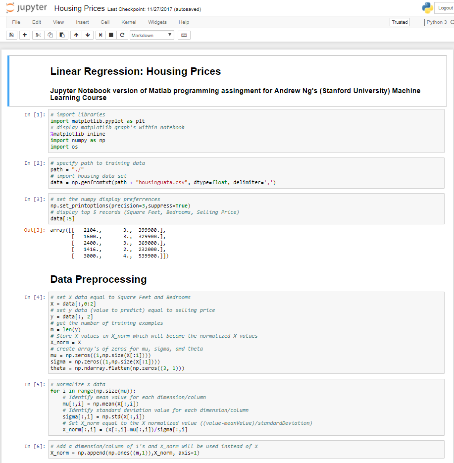
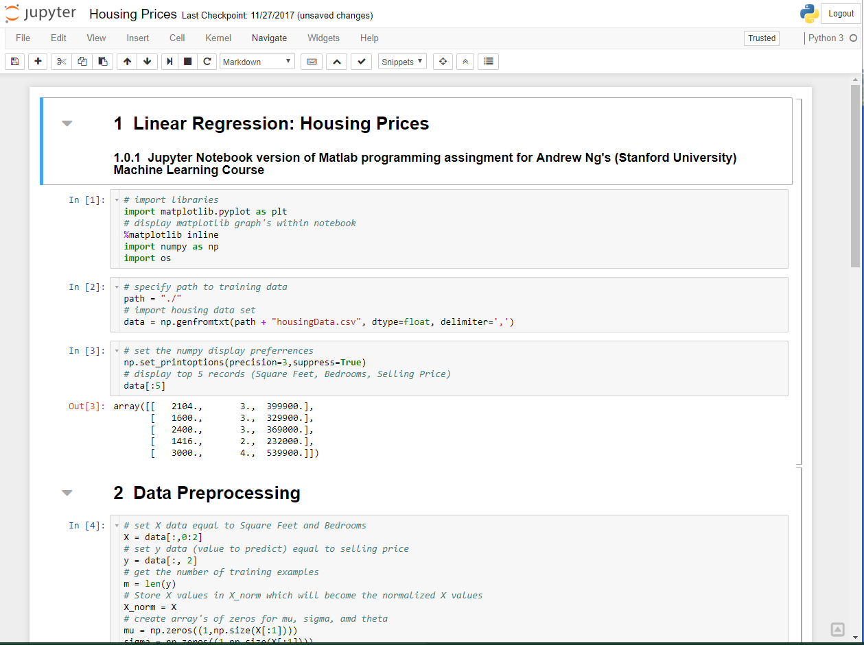
Linear Regression: Housing Prices

Jupyter Notebook version of Matlab programming assingment for Andrew Ng's (Stanford University) Machine Learning Course

# import libraries
import matplotlib.pyplot as plt
# display matplotlib graph's within notebook
%matplotlib inline 
import numpy as np
import os

# specify path to training data
path = "./"
# import housing data set
data = np.genfromtxt(path + "housingData.csv", dtype=float, delimiter=',')

# set the numpy display preferrences
np.set_printoptions(precision=3,suppress=True)
# display top 5 records (Square Feet, Bedrooms, Selling Price)
data[:5]

array([[   2104.,       3.,  399900.],
       [   1600.,       3.,  329900.],
       [   2400.,       3.,  369000.],
       [   1416.,       2.,  232000.],
       [   3000.,       4.,  539900.]])

Data Preprocessing

# set X data equal to Square Feet and Bedrooms
X = data[:,0:2]
# set y data (value to predict) equal to selling price
y = data[:, 2]
# get the number of training examples
m = len(y)
# Store X values in X_norm which will become the normalized X values
X_norm = X
# create array's of zeros for mu, sigma, amd theta
mu = np.zeros((1,np.size(X[:1])))
sigma = np.zeros((1,np.size(X[:1])))
theta = np.ndarray.flatten(np.zeros((3, 1)))

# Normalize X data
for i in range(np.size(mu)):
    # Identify mean value for each dimension/column
    mu[:,i] = np.mean(X[:,i])
    # Identify standard deviation value for each dimension/column
    sigma[:,i] = np.std(X[:,i])
    # Set X_norm equal to the X normalized value ((value-meanValue)/standardDeviation)
    X_norm[:,i] = (X[:,i]-mu[:,i])/sigma[:,i]

# Add a dimension/column of 1's and X_norm will be used instead of X
X_norm = np.append(np.ones((m,1)),X_norm, axis=1)

# Display normalized X data (appended 1's, normalized square footage, normalized bedrooms)
X_norm[:5]

array([[ 1.   ,  0.131, -0.226],
       [ 1.   , -0.51 , -0.226],
       [ 1.   ,  0.508, -0.226],
       [ 1.   , -0.744, -1.554],
       [ 1.   ,  1.271,  1.102]])

Perform Linear Regression

# set learning rate
alpha = 0.01
# set number of interations
num_iters = 400

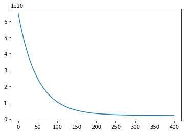
# create blank array to capture cost function value after each iteration
J_history = np.zeros((num_iters, 1))

# perform linear regression for specified number of iterations
for i in range(num_iters):
    theta = theta - np.dot(np.transpose(X_norm),np.ndarray.flatten(np.dot(X_norm,theta)) - y)*(alpha/m)
    # set cost function value to 0 for each iteration
    J_cost = 0
    # capture cost function value across data set
    for j in range(m):
        J_cost = J_cost + ((1/(2*m))*np.square(np.dot(np.transpose(theta),np.transpose(X_norm[j,:]))-y[j]))
    # store cost function value for each itteration
    J_history[i] = J_cost

# display cost function value for each itteration
plt.plot(J_history)

[<matplotlib.lines.Line2D at 0x7ff3d2410f28>]

Predict Selling Price

# set square footage and number of bedrooms to predict selling price
sqrFtPred = 1650
bedRoomPred = 3

# predict selling cost (y value)
predictValues = ([1,(sqrFtPred-mu[0,0])/sigma[0,0],(bedRoomPred-mu[0,1])/sigma[0,1]])
predictedSellingPrice = np.dot(predictValues,theta)

# display predicted selling price
predictedSellingPrice
print('${:,.2f}'.format(predictedSellingPrice))

$289,221.65

Deep Learning Training Resources

Listed below are two invaluable online training resources for deep learning.

• Machine Learning - Andrew Ng (Stanford University) 
  • https://www.coursera.org/learn/machine-learning 
• Practical Deep Learning for Coders - Jeremy Howard
  • http://course.fast.ai/

Overview of Neural Networks and Gradient Descent

Below are a couple videos that provide great overviews of neural networks and gradient descent. Even for those familiar with both topics, these videos are well put together and worth the view. 

Videos by 3Blue1Brown

But what *is* a Neural Network? | Deep learning, Part 1

Gradient descent, how neural networks learn | Deep learning, part 2

Kaggle - Digit Recognizer - CNN 99.4% Accuracy

Imaged below is the basic Convolutional Neural Network (CNN) for the Kaggle - Digit Recognizer competition.

Digit Recognizer - Convolutional Neural Network

Below provides an overview ensembling the CNN model. With executing the fit_model function 5 times, a total of a 125 epochs were executed.

Running predictions against the test set for each model and averaging the prediction for each image.

After exporting and submitting results, the basic CNN achieved 99.4% accuracy.

Kaggle - Invasive Species Monitoring - Ensemble with ROC of 0.95532

Ensemble (Bucket of models) multiple models to achieve ROC of 0.95532.

Below is an example of creating 4 models that were trained for 100 epochs each. The last section of code saves the weights for each model in the set. 

Each model was then used to predict the test image set. The mean prediction for each image was then used for the Kaggle Invasive Species Monitoring competition submission.

Kaggle - Leaf Classification: Directory Structure and Moving Files

Jupyter notebook for setting up the directory structure for Kaggle's Leaf Classification competition has been published. The notebook walks through the process for:

• Unpacking/Unzipping the competition files
• Creating directory structure based off the train.csv data set
• Moving images to appropriate train, valid, and test directories.
  • The train and valid directories contain directories specific to each leaf species

Resolving "The cuda backend is deprecated..." Warning

When using Theano backend, the following warning message was displayed in my Jupyter notebook:

The cuda backend is deprecated and will be removed in the next release (v0.10). Please switch to the gpuarray backend.

The warning message was resolved by completing the following 2 actions:

Action 1. Update Theano config file

1. In Linux terminal execute command
   sudo nano ~/.theanorc
2. Update "device = gpu" to
   device = cuda0

Action 2: Update Jupyter notebook to include "import theano.gpuarray"

Note that the Cuda backend warning message is no longer displayed.

Installing Kaggle CLI and Competition Data Download

In the computer terminal enter the following commands to install the unofficial Kaggle CLI (Command Line Interface) and download competition files:

1. pip install kaggle-cli
2. kg config -u [Kaggle username] -p [Kaggle password]
3. cd Documents/nbs/
4. kg download -c [Kaggle competition name]

The purpose of each command:

1. Installs the Kaggle CLI
2. Sets the username and password for the Kaggle CLI. This is why the username and password parameters do not need defined in step 4.
3. Change computer directory to the location where the competition files will be stored
4. Downloads the competition files. IMPORTANT! before being able to download the competition files, the competition rules will need to be accepted. The accept option is at the end of the rules section of the competition on the Kaggle website

Example of installing Kaggle CLI and downloading Dogs vs. Cats competition files:

1. pip install kaggle-cli
2. kg config -u KaggleUser -p P@ssw0rd123
3. cd Documents/nbs/
4. kg download -c 'dogs-vs-cats'

Operating System Setup

After installing Ubuntu operating system, the following commands were executed in the terminal:

If operating system is earlier release than 16.04 LTS
sudo do-release-upgrade

--optional start
Install SSH Server in order to remote into the deep learning PC from another computer on the same network.
sudo apt-get install openssh-server -y

Verify SSH service is running.
sudo service ssh status

Identify network IP address for SSH client. A populate SSH client is Putty
ifconfig
--optional end

Install Tmux. Useful for operating multiple terminal windows from within the same SSH session. Google Tmux for more information
sudo apt-get install tmux

Update and reboot Ubuntu operating system
sudo apt-get update
sudo apt-get upgrade -y
sudo apt-get dist-upgrade -y
sudo reboot

Installing Anaconda for Ubuntu
cd /tmp
curl -O https://repo.continuum.io/archive/Anaconda3-4.4.0-Linux-x86_64.sh
bash Anaconda3-4.4.0-Linux-x86_64.sh
[enter] and [yes] to all
sudo reboot

After Anaconda is installed, configure Jupyter notebooks.
jupyter notebook --generate-config
[note config location]
jupyter notebook password
[enter password]
sudo nano /home/cnnpc/.jupyter/jupyter_notebook_config.py
Change #c.NotebookApp.ip = 'localhost' to c.NotebookApp.ip = '[your ip]'
Change #c.NotebookApp.port = 8888 to c.NotebookApp.port = [your port]

Create a Jupyter notebook directory in your Documents directory
cd Documents/
mkdir nbs
cd nbs
jupyter notebook
[verify and connect]

Install Nvidia repos and Cuda
cd /tmp
wget "http://developer.download.nvidia.com/compute/cuda/repos/ubuntu1604/x86_64/cuda-repo-ubuntu1604_8.0.44-1_amd64.deb" -O "cuda-repo-ubuntu1604_8.0.44-1_amd64.deb"
sudo dpkg -i cuda-repo-ubuntu1604_8.0.44-1_amd64.deb
sudo apt-get update
sudo apt-get -y install cuda
sudo reboot
sudo modprobe nvidia

Verify GPU is recognized
nvidia-smi

Install bcolz and pip.
conda install -y bcolz
sudo apt-get install python3-pip -y

Upgrade Anaconda modules
conda upgrade -y --all

Install Keras
pip install keras==1.2.2

Create Keras directory
mkdir ~/.keras

Create Keras json configuration file. (copy echo.. ..keras.json and paste into terminal and press enter)
echo '{
"image_dim_ordering": "th",
"epsilon": 1e-07,
"floatx": "float32",
"backend": "theano"
}' > ~/.keras/keras.json

Install Theano
pip3 install theano

Create Theano configuration file. (copy echo.. ..theanorc and paste into terminal and press enter)
echo "[global]
device = gpu
floatX = float32
[cuda]
root = /usr/local/cuda" > ~/.theanorc

Install Theano pygpu
conda install theano pygpu

Get fast.ai cudnn file, extract, and copy to appropriate directories
wget "http://files.fast.ai/files/cudnn.tgz" -O "cudnn.tgz"
tar -zxf cudnn.tgz
cd cuda
sudo cp lib64/* /usr/local/cuda/lib64/
sudo cp include/* /usr/local/cuda/include/

Install Glances. This is a great application for monitoring computer usage. (Including GPU usage)
curl -L https://bit.ly/glances | /bin/bashsudo

Deep Learning PC Build

List of parts for a deep learning capable PC for around $1000 USD:

• Intel Core i5-7500
  • $  198.03 Amazon
• Ballistix Sport LT 16GB Kit
  • $  135.95 Amazon
• EVGA SuperNOVA 650 G2
  • $  108.89 Amazon
• GIGABYTE GA-H270-HD3
  • $    99.99 Amazon
• Corsair Carbide Series SPEC-01
  • $    58.99 Amazon
• Samsung 850 EVO 250GB 2.5-Inch SATA III Internal SSD
  • $    89.99 Amazon
• GEFORCE GTX 1060 6GB
  • $  299.00 Nvidia

Parts not listed:

• PC Monitor
• Keyboard and Mouse
• 4 GB or greater USB drive