Linear Regression: Housing Prices (Andrew Ng - Stanford University)

Below is an example of linear regression performed within a Jupyter notebook. This simple linear regression notebook was built to mirror a Matlab linear regression project in Andrew Ng's Stanford University Machine Learning course. The python Jupyter notebook can be downloaded here and the data set used can be downloaded here.

Linear Regression: Housing Prices

Jupyter Notebook version of Matlab programming assingment for Andrew Ng's (Stanford University) Machine Learning Course

# import libraries
import matplotlib.pyplot as plt
# display matplotlib graph's within notebook
%matplotlib inline 
import numpy as np
import os

# specify path to training data
path = "./"
# import housing data set
data = np.genfromtxt(path + "housingData.csv", dtype=float, delimiter=',')

# set the numpy display preferrences
np.set_printoptions(precision=3,suppress=True)
# display top 5 records (Square Feet, Bedrooms, Selling Price)
data[:5]

array([[   2104.,       3.,  399900.],
       [   1600.,       3.,  329900.],
       [   2400.,       3.,  369000.],
       [   1416.,       2.,  232000.],
       [   3000.,       4.,  539900.]])

Data Preprocessing

# set X data equal to Square Feet and Bedrooms
X = data[:,0:2]
# set y data (value to predict) equal to selling price
y = data[:, 2]
# get the number of training examples
m = len(y)
# Store X values in X_norm which will become the normalized X values
X_norm = X
# create array's of zeros for mu, sigma, amd theta
mu = np.zeros((1,np.size(X[:1])))
sigma = np.zeros((1,np.size(X[:1])))
theta = np.ndarray.flatten(np.zeros((3, 1)))

# Normalize X data
for i in range(np.size(mu)):
    # Identify mean value for each dimension/column
    mu[:,i] = np.mean(X[:,i])
    # Identify standard deviation value for each dimension/column
    sigma[:,i] = np.std(X[:,i])
    # Set X_norm equal to the X normalized value ((value-meanValue)/standardDeviation)
    X_norm[:,i] = (X[:,i]-mu[:,i])/sigma[:,i]

# Add a dimension/column of 1's and X_norm will be used instead of X
X_norm = np.append(np.ones((m,1)),X_norm, axis=1)

# Display normalized X data (appended 1's, normalized square footage, normalized bedrooms)
X_norm[:5]

array([[ 1.   ,  0.131, -0.226],
       [ 1.   , -0.51 , -0.226],
       [ 1.   ,  0.508, -0.226],
       [ 1.   , -0.744, -1.554],
       [ 1.   ,  1.271,  1.102]])

Perform Linear Regression

# set learning rate
alpha = 0.01
# set number of interations
num_iters = 400

# create blank array to capture cost function value after each iteration
J_history = np.zeros((num_iters, 1))

# perform linear regression for specified number of iterations
for i in range(num_iters):
    theta = theta - np.dot(np.transpose(X_norm),np.ndarray.flatten(np.dot(X_norm,theta)) - y)*(alpha/m)
    # set cost function value to 0 for each iteration
    J_cost = 0
    # capture cost function value across data set
    for j in range(m):
        J_cost = J_cost + ((1/(2*m))*np.square(np.dot(np.transpose(theta),np.transpose(X_norm[j,:]))-y[j]))
    # store cost function value for each itteration
    J_history[i] = J_cost

# display cost function value for each itteration
plt.plot(J_history)

[<matplotlib.lines.Line2D at 0x7ff3d2410f28>]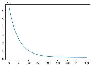

Predict Selling Price

# set square footage and number of bedrooms to predict selling price
sqrFtPred = 1650
bedRoomPred = 3

# predict selling cost (y value)
predictValues = ([1,(sqrFtPred-mu[0,0])/sigma[0,0],(bedRoomPred-mu[0,1])/sigma[0,1]])
predictedSellingPrice = np.dot(predictValues,theta)

# display predicted selling price
predictedSellingPrice
print('${:,.2f}'.format(predictedSellingPrice))

$289,221.65